CS5805 - Probability Theory

Hidden Markov Models (HMMs) are a powerful statistical tool used in various fields, including speech recognition, bioinformatics, and natural language processing. Grounded in probability theory, HMMs are a type of stochastic model that represents a system evolving over time with hidden states. The model assumes that the observed data result from a probabilistic process involving these hidden states, making it particularly effective in situations where the underlying dynamics are not directly observable but can be inferred through observed data and the probabilities governing state transitions and emissions. Probability theory forms the backbone of HMMs, allowing them to make predictions and decisions based on the likelihood of sequences of observations given the model’s parameters.

Code

import numpy as np
import pandas as pd
import matplotlib.pyplot as plt
%matplotlib inline
import warnings
warnings.filterwarnings("ignore")

The hmmlearn library in Python performs Unsupervised learning and inference of Hidden Markov Models.

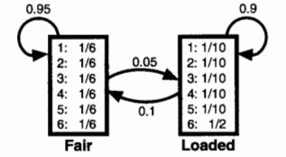
Let us take the common Hidden Markov Model example of the ocassionally dishonest casino. In a casino, they use a fair die most of the time, but switch to the loaded die once in a while. The purpose of making use of the Hidden Markov Model is to identify instances when the dice roll is probabilistically from the fair die or the loaded die.

The probabilities for the various outcome variables have been adapted from this textbook.

The emission probabilities are the probability of each outcome (die roll) at its current state. The transition probabilities define the probability of transitioning to a state (fair, loaded), and the start probabilities define the starting probability of being in each state.

From the hmmlearn library, the CategoricalHMM model (derived from the MultinomialHMM model), uses the Baum-Welch algorithm for training hidden Markov models (HMMs). The Baum-Welch algorithm, also known as the Forward-Backward algorithm or the Expectation-Maximization (EM) algorithm for HMMs, is an iterative procedure for estimating the parameters of an HMM given a set of observed data.

You can read more on the training of the Hidden Markov Model and the probability theory behind identifying the sequence state part at the end of this blog.

In the block of code below, we initialize the probabilities, initialize the CategoricalHMM method which takes in n_components as the number of possible states, the number of iterations for training. The other parameters (such as init_param, algorithm, etc.) details can be found here.

We then use the sample() method to generate die roll and corresponding state samples.

from hmmlearn import hmm

gen_model = hmm.CategoricalHMM(n_components=2, n_iter=100, init_params = 'se')

gen_model.startprob_ = np.array([1.0, 0.0])

gen_model.transmat_ = np.array([[0.95, 0.05],
                                [0.1, 0.9]])

gen_model.emissionprob_ = \
    np.array([[1 / 6, 1 / 6, 1 / 6, 1 / 6, 1 / 6, 1 / 6],
              [1 / 10, 1 / 10, 1 / 10, 1 / 10, 1 / 10, 1 / 2]])

rolls, gen_states = gen_model.sample(30000)

Transition Model:
Emission Matrix:

	Fair	Unfair
1	0.166667	0.1
2	0.166667	0.1
3	0.166667	0.1
4	0.166667	0.1
5	0.166667	0.1

Sample of Dice Rolls generated

	Roll	Coin_State
0	1	0
1	4	0
2	5	0
3	1	0
4	1	0

Plotting the states of the first 500 generated coin flips:

Code

fig, ax = plt.subplots()
ax.plot(gen_states[:500])
ax.set_title('States over time')
ax.set_xlabel('Time (# of rolls)')
ax.set_ylabel('State')
fig.show()

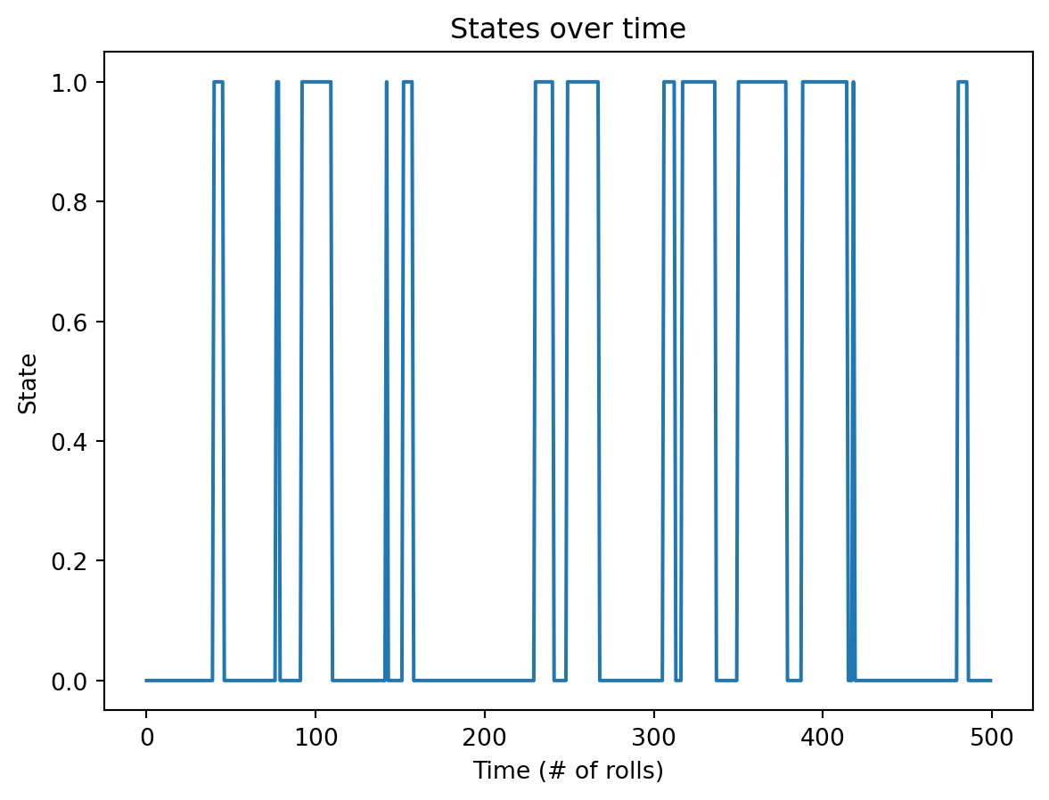
Plotting the rolls for the fair and loaded states

Code

fig, ax = plt.subplots()
ax.hist(rolls[gen_states == 0], label='fair', alpha=0.5,
        bins=np.arange(7) - 0.5, density=True)
ax.hist(rolls[gen_states == 1], label='loaded', alpha=0.5,
        bins=np.arange(7) - 0.5, density=True)
ax.set_title('Roll probabilities by state')
ax.set_xlabel('Count')
ax.set_ylabel('Roll')
ax.legend()
fig.show()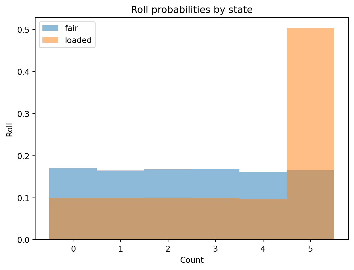

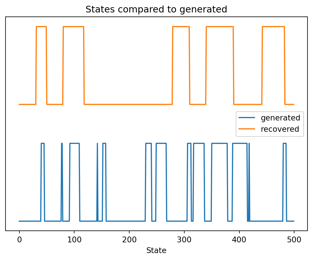
In the code below, we are performing a 50%-50% train-test dataset split. We are then fitting the model on our train set and obtaining the score for the model which is simply the log probability under the model. Then, we make use of the predict method which implements the Viterbi algorithm to predict the best sequence of states for the given observations (dice rolls).

# split our data into training and validation sets (50/50 split)
X_train = rolls[:rolls.shape[0] // 2]
X_test = rolls[rolls.shape[0] // 2:]
y_test = np.array(gen_states[gen_states.shape[0] // 2:])
gen_model = gen_model.fit(X_train)

# check base score (non-tuned model)
gen_score = gen_model.score(X_test)

print(f'Generated score: {gen_score}')

# use the Viterbi algorithm to predict the most likely sequence of states
# given the model
states = gen_model.predict(X_test)

Even though the 'startprob_' attribute is set, it will be overwritten during initialization because 'init_params' contains 's'
Even though the 'emissionprob_' attribute is set, it will be overwritten during initialization because 'init_params' contains 'e'

Generated score: -26111.908215770163

Recovered states vs Generated states:

Code

fig, ax = plt.subplots()
ax.plot(gen_states[:500], label='generated')
ax.plot(states[:500] + 1.5, label='recovered')
ax.set_yticks([])
ax.set_title('States compared to generated')
ax.set_xlabel('Time (# rolls)')
ax.set_xlabel('State')
ax.legend()
fig.show()

Updated Markov Model probabilities after training the HMM on the dataset with the Baum-Welch algorithm.

Transition Model:
Emission Matrix: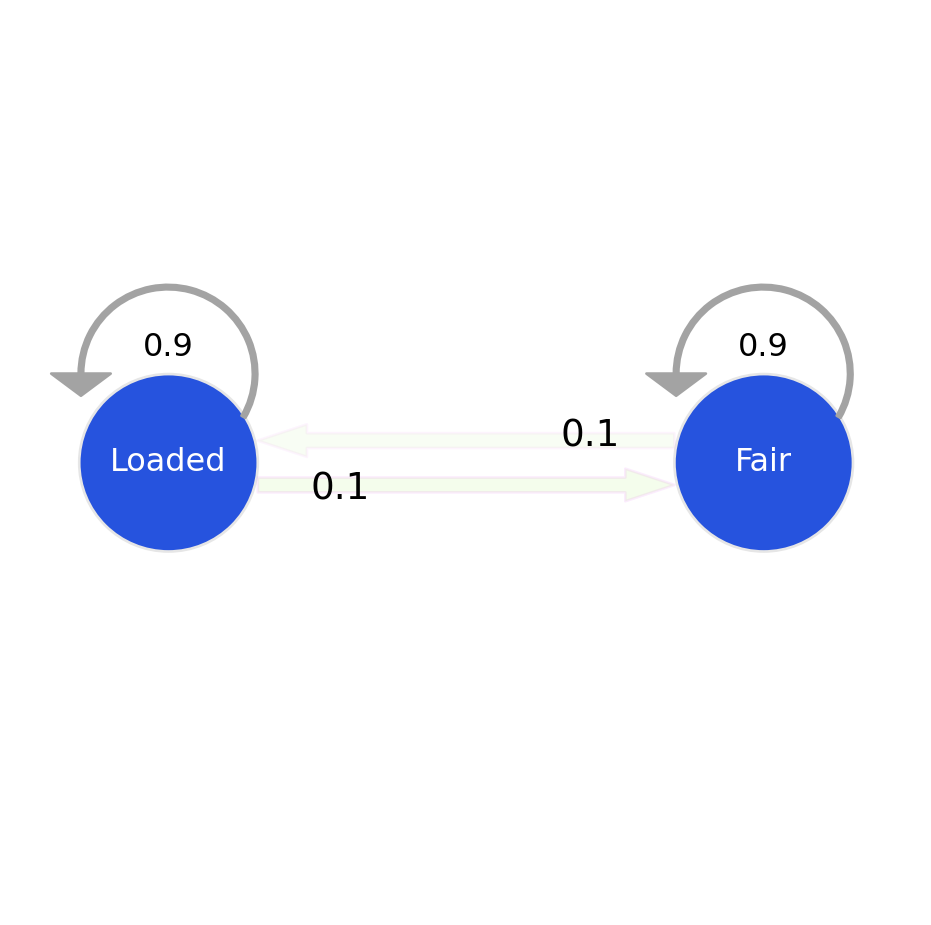

	Fair	Unfair
1	0.170	0.100
2	0.168	0.096
3	0.165	0.111
4	0.164	0.104
5	0.171	0.094

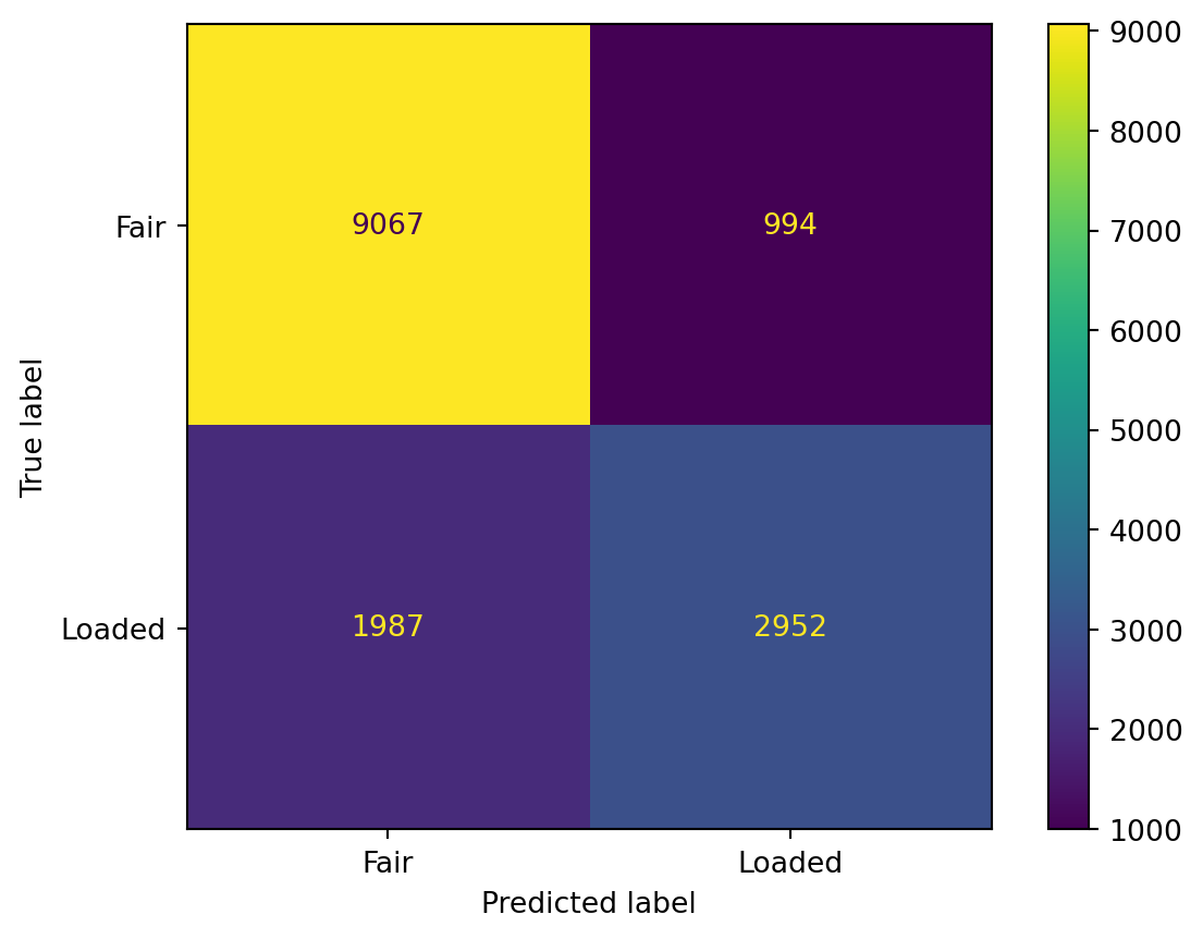
Results of the model in the form of a confusion matrix to identify how many times the model predicted ‘Fair’ and ‘Loaded’ coin correctly given the dice roll.

As we can see from the results below, the accuracy of the model is not considered to be extremely good. This is because we are dealing with a truly probabilistic model, the results are based on the ‘likelihood’ parameter. Also, the model has been trained on sample data which may not mimic true data to the fullest.

Code

from sklearn.metrics import confusion_matrix, classification_report, ConfusionMatrixDisplay
from sklearn.metrics import RocCurveDisplay

# True states (hidden states)
true_states = y_test
predicted_states = states

# Evaluate confusion matrix
conf_matrix = confusion_matrix(true_states, predicted_states)
# Display confusion matrix
print("Confusion Matrix:")
disp = ConfusionMatrixDisplay(confusion_matrix=conf_matrix, display_labels=['Fair', 'Loaded'])
disp.plot()
plt.show()

# Evaluate classification report
class_report = classification_report(true_states, predicted_states)

# Display classification report
print("Classification Report:")
print(class_report)

RocCurveDisplay.from_predictions(true_states, predicted_states)

Confusion Matrix:
Classification Report:
              precision    recall  f1-score   support

           0       0.82      0.90      0.86     10061
           1       0.75      0.60      0.66      4939

    accuracy                           0.80     15000
   macro avg       0.78      0.75      0.76     15000
weighted avg       0.80      0.80      0.79     15000

<sklearn.metrics._plot.roc_curve.RocCurveDisplay at 0x2911d9aad70>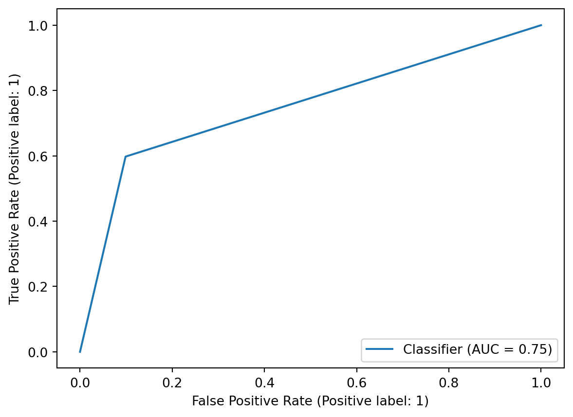

Code

def convert_to_numpy(string_val, type):
    str_int = []
    if type == "rolls":
        for i in string_val:
            str_int.append(np.array([int(i)-1]))
    else:
        dice = {'F':0, 'L':1}
        for i in string_val:
            str_int.append(np.array(dice[i]))
    return str_int

def convert_to_string(string_die):
    dice = {0: 'F', 1:'L'}
    string = ""
    for i in string_die:
        string+=dice[i]
    return string

Testing the model on an example taken from the textbook: {width = 60%}

Code

test_rolls1 = "315116246446644245311321631164152133625144543631656626566666"

y_true1 = "FFFFFFFFFFFFFFFFFFFFFFFFFFFFFFFFFFFFFFFFFFFFFFFFLLLLLLLLLLLL"

test_rolls2 = "222555441666566563564324364131513465146353411126414626253356"
y_true2 = "FFFFFFFFLLLLLLLLLLLLLFFFFFFFFFFFFFFFFFFFFFFFFFFFFFFFFFFFFFFL"

X_test_1 = convert_to_numpy(test_rolls1, "rolls")
y_test_1 = gen_model.predict(X_test_1)
b = convert_to_string(y_test_1)
print(f"Output:{test_rolls1} \nDie:{y_true1} \nViterbi:{b}")

X_test_2 = convert_to_numpy(test_rolls2, "rolls")
y_test_2 = gen_model.predict(X_test_2)
b = convert_to_string(y_test_2)
print(f"Output:{test_rolls2} \nDie:{y_true2} \nViterbi:{b}")

Output:315116246446644245311321631164152133625144543631656626566666 
Die:FFFFFFFFFFFFFFFFFFFFFFFFFFFFFFFFFFFFFFFFFFFFFFFFLLLLLLLLLLLL 
Viterbi:FFFFFFFFFFFFFFFFFFFFFFFFFFFFFFFFFFFFFFFFFFFFFLLLLLLLLLLLLLLL
Output:222555441666566563564324364131513465146353411126414626253356 
Die:FFFFFFFFLLLLLLLLLLLLLFFFFFFFFFFFFFFFFFFFFFFFFFFFFFFFFFFFFFFL 
Viterbi:FFFFFFFFFFFFFFFFFFFFFFFFFFFFFFFFFFFFFFFFFFFFFFFFFFFFFFFFFFFF

Detailing the probability theory behind the Hidden Markov Model The Baum-Welch algorithm, also known as the Forward-Backward algorithm, is a parameter estimation technique for Hidden Markov Models (HMMs). Named after Leonard Baum and Lloyd Welch, this algorithm is a form of the Expectation-Maximization (EM) algorithm. Its primary goal is to iteratively refine the parameters of an HMM based on observed data, making it a powerful tool for model training.

The algorithm consists of two main steps, the expectation step and the maximization step.

The parameters of a HMM are given by $\theta=(A,B,\pi)$, where:

$A$ is the state transition matrix, which defines the probability of transitioning from one state to another.
$B$ is the emission matrix, which defines the probability of emitting a given observation from a given state.
$\pi$ is the initial state distribution, which defines the probability of being in each state at the beginning of the sequence.

$A=\{a_{ij}\}=P(X_{t}=j|X_{t-1}=i)$ is the state transition matrix

$\pi=\{\pi_{i}\}=P(X_{1}=i)$ is the initial state distribution

$B=\{b_{j}(y_{t})\}=P(Y_{t}=y_{t}|X_{t}=j)$ is the emission matrix

Given observation sequences $(Y=(Y_{1}=y_{1},Y_{2}=y_{2},...,Y_{T}=y_{T}))$ the algorithm tries to find the parameters $(\theta)$ that maximise the probability of the observation.

The algorithm starts by choosing some initial values for the HMM parameters $\theta = (A, B, \pi)$. Then, it repeats the following steps until convergence:

Determine probable state paths. This involves calculating the probability of each possible state path, given the observed sequence of emissions.
Count the expected number of transitions and emissions. This involves counting the number of times each state transition is taken and each emission is made, weighted by the probability of each state path.
Re-estimate the HMM parameters. This involves using the expected number of transitions and emissions to update the HMM parameters $\theta$.

The forward-backward algorithm is used for finding probable paths.

Forward Procedure $(\alpha_{i}(t)=P(Y_{1}=y_{1},...,Y_{t}=y_{t},X_{t}=i|\theta))$ be the probability of seeing $(y_{1},...,y_{t})$ and being in state $i$ at time $t$. Found recursively using:

$\(\alpha_{i}(1)=\pi_{i}b_{i}(y_{1})$\)

$\(\alpha_{j}(t+1)=b_{j}(y_{t+1})\sum_{i=1}^{N}\alpha_{i}(t)a_{ij}$\)

Backward Procedure $(\beta_{i}(t)=P(Y_{t+1}=y_{t+1},...,Y_{T}=y_{T}|X_{t}=i,\theta))$ be the probability of ending partial sequence $(y_{t+1},...,y_{T})$ given starting state $i$ at time $t$.

$(\beta_{i}(t))$ is computed recursively as:

$\(\beta_{i}(T)=1$\) $\(\beta_{i}(t)=\sum_{j=1}^{N}\beta_{j}(t+1)a_{ij}b_{j}(y_{t+1}))$

Code

def forward(states, sequence, a, b, pi, key):
    N = len(states)
    T = len(sequence)
    pi = pi[key] # prob of state i, since 2 states, let's half it be 0.5, 0.5 initially
    i = key # holds the first state

    # Pseudocount to handle zeros
    pseudocount = 1e-100
    # for all possible states, and the first actual state (alpha)
    # i.e. alpha i for all i has been caluclated given yt
    alpha = np.zeros((N, T))
    alpha[:,0] = pi * b[:,int(sequence[0])] + pseudocount


    # next, we have to do iterations to calculate alpha at different times t
    # we need all alpha values since it is going to be summed up to calculate gamma
    
    for t in range(1, T):
        for j in range(N):
            alpha[j][t] = sum(alpha[i][t-1]*a[i][j]*b[j][int(sequence[t])] for i in range(N)) + pseudocount

    return alpha

Code

def backward(states, sequence, a, b):
    N = len(states)
    T = len(sequence)
    beta = np.zeros((N, T))

    # Pseudocount to handle zeros
    pseudocount = 1e-100

    # Initialization
    beta[:, -1] = 1  # Set the last column to 1

    # Recursion
    for t in range(T - 2, -1, -1):
        for i in range(N):
            beta[i, t] = sum(a[i, j] * b[j, int(sequence[t + 1])] * beta[j, t + 1] for j in range(N)) + pseudocount

    return beta

The Expectation step: Calculate the probabilities of being in each state at each time step given the observed sequence using the Forward-Backward algorithm. These probabilities represent the likelihood of the system being in state $i$ at time $t$ given the entire observed sequence. Calculate the joint probabilities of transitioning from state $i$ to state $j$ at consecutive time steps given the observed sequence.

$\gamma_t(i) = \frac{\alpha_t(i) \cdot \beta_t(i)}{\sum_{j=1}^{N} \alpha_t(j) \cdot \beta_t(j)}$

$\xi_t(i, j) = \frac{\alpha_t(i) \cdot a_{ij} \cdot b_j(o_{t+1}) \cdot \beta_{t+1}(j)}{\sum_{k=1}^{N} \sum_{l=1}^{N} \alpha_t(k) \cdot a_{kl} \cdot b_l(o_{t+1}) \cdot \beta_{t+1}(l)}$

The Maximization step: Update the model parameters, including the initial state probabilities, transition probabilities, and emission probabilities. The updated parameters are computed by normalizing the expected counts derived from the E-step.

$\hat{\pi}_i = \gamma_1(i)$

$\hat{a}_{ij} = \frac{\sum_{t=1}^{T-1} \xi_t(i, j)}{\sum_{t=1}^{T-1} \gamma_t(i)}$

$\hat{b}_i(k) = \frac{\sum_{t=1}^{T} \gamma_t(i) \cdot \delta_{o_t, k}}{\sum_{t=1}^{T} \gamma_t(i)}$

Code

def train(a, b, pi, sequence, states, key, n_iterations = 100, tol=1e-6):
    #Baum-Welch algorithm for HMM
    # calculate gamma, xi, and then update a and b parameters
    N = len(states)
    T = len(sequence)
    
    # M is the number of possible observations i.e. number of columns
    M = b.shape[1]

    prev_log_likelihood = 0

    for iteration in range(n_iterations):
        alpha = forward(states, sequence, a, b, pi, key)
        beta = backward(states, sequence, a, b)

        print(f"Alpha: {alpha}")
        print(f"Beta:{beta}")

        # Pseudocount to handle zeros
        pseudocount = 1e-100
        gamma = alpha * beta
        # print(gamma)
        denominator = np.sum(gamma, axis=0, keepdims=True) # same for all i
        gamma = gamma/denominator + pseudocount

        print(f"gamma:{gamma}") 

        xi = np.zeros((N, N, T - 1))

        for i in range(N):
            for j in range(N):
                for t in range(T - 1):
                    numerator = alpha[i, t] * a[i, j] * b[j, int(sequence[t + 1])] * beta[j, t + 1]
                    denominator = np.sum(alpha[k, t] * a[k, l] * b[l, int(sequence[t + 1])] * beta[l, t + 1] for k in range(N) for l in range(N))
                    xi[i, j, t] = (numerator / denominator) + pseudocount

        print(f"Xi: {xi}")


        # update a and b
        # M-step
        '''
        sequence == k creates a boolean array of the same length as sequence, where each element is True if the corresponding element in sequence is equal to k, and False otherwise.
    mask = (sequence == k) assigns this boolean array to the variable mask.
    In the context of the Baum-Welch algorithm or similar algorithms for Hidden Markov Models (HMMs), this kind of mask is often used to select specific observations in the computation of probabilities. For example, 
    it might be used to sum over only the observations that match a particular value, which is relevant when updating the emission matrix b.
        '''
        # a = (np.sum(xi, axis=2) + pseudocount)/ np.sum(gamma[:, :-1], axis=1, keepdims=True) 
        for i in range(N):  # N is the number of states
            for j in range(N):  # N is the number of states
                numerator = np.sum(xi[i, j, :])
                denominator = np.sum(gamma[i, :])
                a[i, j] = (numerator+pseudocount) / (denominator+pseudocount) 


        b = np.zeros((N, M))
        # print(gamma.shape)
        gamma_sum = np.sum(gamma, axis=1)
        
        obs = []
        for i in sequence:
            obs.append(int(i))
        obs = np.array(obs)

        for j in range(N):
            for k in range(M):
                mask = (obs==k) # for indicative function i.e. 1 if observed = yt, else 0
                b[j, k] = (np.sum(gamma[j]*mask)+ pseudocount) / (np.sum(gamma[j]) + pseudocount) 
        

        # Normalize rows to ensure each row sums to 1.0
        a = a / np.sum(a, axis=1)[:, np.newaxis]
        b = b / np.sum(b, axis=1)[:, np.newaxis]

        print(f"a = {a}, b = {b}")

        # Log Likelihood Calculation
        log_likelihood = np.sum(np.log(np.sum(alpha, axis=0)))

        # Convergence Check
        if np.abs(log_likelihood - prev_log_likelihood) < tol:
            print(f"Converged after {iteration + 1} iterations.")
            break

        prev_log_likelihood = log_likelihood

    return a, b, pi

The Viterbi algorithm is a dynamic programming algorithm used for decoding Hidden Markov Models (HMMs) and finding the most likely sequence of hidden states given an observed sequence. The algorithm efficiently determines the optimal state sequence by considering the probabilities of transitions and emissions.

The core idea behind the Viterbi algorithm is to iteratively compute the most likely path to each state at each time step, incorporating both the current observation and the previously calculated probabilities.

\[ δ_i(t) = max_j δ_j(t - 1) a_ji b_i(Y_t) \]

\[ ψ_i(t) = argmax_j δ_j(t - 1) a_ji \]

Code

def predict(sequence, states, a, b, pi):
    # Makes use of the viterbi algorithm to predict best path
    # Initialize Variables
    T = len(sequence)
    N = len(states)

    # Pseudocount to handle zeros
    pseudocount = 1e-100

    viterbi_table = np.zeros((N, T)) # delta
    backpointer = np.zeros((N, T)) # psi

    # Initialization step, for t = 0
    print(int(sequence[0]))
    viterbi_table[:, 0] = pi * b[:, int(sequence[0])] + pseudocount

    # Calculate Probabilities
    for t in range(1, T):
        for s in range(N):
            
            max_prob = max(viterbi_table[prev_s][t-1] * a[prev_s][s] for prev_s in range(N)) * b[s][int(sequence[t])] 
            viterbi_table[s][t] = max_prob + pseudocount
            backpointer[s][t] = np.argmax([viterbi_table[prev_s][t-1] * a[prev_s][s]for prev_s in range(N)])

    #Traceback and Find Best Path
    best_path = []
    last_state = np.argmax(viterbi_table[:, -1])

    best_path.append(last_state)
    best_prob = 1.0
    for t in range(T-2, -1, -1):
        last_state = last_state = np.argmax(viterbi_table[:, t])
        best_prob *= (viterbi_table[last_state, t] + pseudocount)
        best_path.append(last_state) # i.e. add to start of list

        
    return best_path

Hidden Markov Models are also used in many applications, one such interesting one is to identify cpgIslandsgiven a genomic sequence. You can read more about it here!.

--- title: "Probability Theory" author: "Anushka S" date: "2023-12-03" categories: [Probability Theory, Machine Learning, Random Variables, Hidden Markov Models, Viterbi algorithm, Baum Welch] --- Hidden Markov Models (HMMs) are a powerful statistical tool used in various fields, including speech recognition, bioinformatics, and natural language processing. Grounded in probability theory, HMMs are a type of stochastic model that represents a system evolving over time with hidden states. The model assumes that the observed data result from a probabilistic process involving these hidden states, making it particularly effective in situations where the underlying dynamics are not directly observable but can be inferred through observed data and the probabilities governing state transitions and emissions. Probability theory forms the backbone of HMMs, allowing them to make predictions and decisions based on the likelihood of sequences of observations given the model's parameters. ```{python} import numpy as np import pandas as pd import matplotlib.pyplot as plt %matplotlib inline import warnings warnings.filterwarnings("ignore") ``` The [hmmlearn](https://hmmlearn.readthedocs.io/en/latest/) library in Python performs Unsupervised learning and inference of Hidden Markov Models. Let us take the common Hidden Markov Model example of the ocassionally dishonest casino. In a casino, they use a fair die most of the time, but switch to the loaded die once in a while. The purpose of making use of the Hidden Markov Model is to identify instances when the dice roll is probabilistically from the fair die or the loaded die. The probabilities for the various outcome variables have been adapted from [this textbook](https://doi.org/10.1017/CBO9780511790492). ![Markov Model for dishonest casino](dice_prob.JPG){width=30%} The emission probabilities are the probability of each outcome (die roll) at its current state. The transition probabilities define the probability of transitioning to a state (fair, loaded), and the start probabilities define the starting probability of being in each state. From the hmmlearn library, the CategoricalHMM model (derived from the MultinomialHMM model), uses the Baum-Welch algorithm for training hidden Markov models (HMMs). The Baum-Welch algorithm, also known as the Forward-Backward algorithm or the Expectation-Maximization (EM) algorithm for HMMs, is an iterative procedure for estimating the parameters of an HMM given a set of observed data. You can read more on the training of the Hidden Markov Model and the probability theory behind identifying the sequence state part at the end of this blog. In the block of code below, we initialize the probabilities, initialize the CategoricalHMM method which takes in n_components as the number of possible states, the number of iterations for training. The other parameters (such as init_param, algorithm, etc.) details can be found [here](https://hmmlearn.readthedocs.io/en/latest/api.html#categoricalhmm). We then use the sample() method to generate die roll and corresponding state samples. ```{python} #| code-fold: false #| code-line-numbers: true from hmmlearn import hmm gen_model = hmm.CategoricalHMM(n_components=2, n_iter=100, init_params = 'se') gen_model.startprob_ = np.array([1.0, 0.0]) gen_model.transmat_ = np.array([[0.95, 0.05], [0.1, 0.9]]) gen_model.emissionprob_ = \ np.array([[1 / 6, 1 / 6, 1 / 6, 1 / 6, 1 / 6, 1 / 6], [1 / 10, 1 / 10, 1 / 10, 1 / 10, 1 / 10, 1 / 2]]) rolls, gen_states = gen_model.sample(30000) ``` ```{python} #| echo: false import matplotlib.pyplot as plt # Import the MarkovChain class from markovchain.py from markovchain import MarkovChain P = gen_model.transmat_ mc = MarkovChain(P, ['Fair', 'Loaded']) print("Transition Model:") mc.draw() data = {'Fair': gen_model.emissionprob_[0], 'Unfair': gen_model.emissionprob_[1]} df_emission = pd.DataFrame(data, index=['1', '2', '3', '4', '5', '6']) print("Emission Matrix:") df_emission.head() ``` ```{python} #| echo: false print("Sample of Dice Rolls generated") pd.DataFrame({'Roll': rolls.flatten()[0:10]+1, 'Coin_State': gen_states.flatten()[0:10]}).head() ``` Plotting the states of the first 500 generated coin flips: ```{python} fig, ax = plt.subplots() ax.plot(gen_states[:500]) ax.set_title('States over time') ax.set_xlabel('Time (# of rolls)') ax.set_ylabel('State') fig.show() ``` Plotting the rolls for the fair and loaded states ```{python} fig, ax = plt.subplots() ax.hist(rolls[gen_states == 0], label='fair', alpha=0.5, bins=np.arange(7) - 0.5, density=True) ax.hist(rolls[gen_states == 1], label='loaded', alpha=0.5, bins=np.arange(7) - 0.5, density=True) ax.set_title('Roll probabilities by state') ax.set_xlabel('Count') ax.set_ylabel('Roll') ax.legend() fig.show() ``` In the code below, we are performing a 50%-50% train-test dataset split. We are then fitting the model on our train set and obtaining the score for the model which is simply the log probability under the model. Then, we make use of the predict method which implements the Viterbi algorithm to predict the best sequence of states for the given observations (dice rolls). ```{python} #| code-fold: false #| code-line-numbers: true # split our data into training and validation sets (50/50 split) X_train = rolls[:rolls.shape[0] // 2] X_test = rolls[rolls.shape[0] // 2:] y_test = np.array(gen_states[gen_states.shape[0] // 2:]) gen_model = gen_model.fit(X_train) # check base score (non-tuned model) gen_score = gen_model.score(X_test) print(f'Generated score: {gen_score}') # use the Viterbi algorithm to predict the most likely sequence of states # given the model states = gen_model.predict(X_test) ``` Recovered states vs Generated states: ```{python} fig, ax = plt.subplots() ax.plot(gen_states[:500], label='generated') ax.plot(states[:500] + 1.5, label='recovered') ax.set_yticks([]) ax.set_title('States compared to generated') ax.set_xlabel('Time (# rolls)') ax.set_xlabel('State') ax.legend() fig.show() ``` Updated Markov Model probabilities after training the HMM on the dataset with the Baum-Welch algorithm. ```{python} #| echo: false import matplotlib.pyplot as plt # Import the MarkovChain class from markovchain.py from markovchain import MarkovChain P = gen_model.transmat_.round(3) mc = MarkovChain(P, ['Fair', 'Loaded']) print("Transition Model:") mc.draw() data = {'Fair': gen_model.emissionprob_.round(3)[0], 'Unfair': gen_model.emissionprob_.round(3)[1]} df_emission = pd.DataFrame(data, index=['1', '2', '3', '4', '5', '6']) print("Emission Matrix:") df_emission.head() ``` Results of the model in the form of a confusion matrix to identify how many times the model predicted 'Fair' and 'Loaded' coin correctly given the dice roll. As we can see from the results below, the accuracy of the model is not considered to be extremely good. This is because we are dealing with a truly probabilistic model, the results are based on the 'likelihood' parameter. Also, the model has been trained on sample data which may not mimic true data to the fullest. ```{python} from sklearn.metrics import confusion_matrix, classification_report, ConfusionMatrixDisplay from sklearn.metrics import RocCurveDisplay # True states (hidden states) true_states = y_test predicted_states = states # Evaluate confusion matrix conf_matrix = confusion_matrix(true_states, predicted_states) # Display confusion matrix print("Confusion Matrix:") disp = ConfusionMatrixDisplay(confusion_matrix=conf_matrix, display_labels=['Fair', 'Loaded']) disp.plot() plt.show() # Evaluate classification report class_report = classification_report(true_states, predicted_states) # Display classification report print("Classification Report:") print(class_report) RocCurveDisplay.from_predictions(true_states, predicted_states) ``` ```{python} def convert_to_numpy(string_val, type): str_int = [] if type == "rolls": for i in string_val: str_int.append(np.array([int(i)-1])) else: dice = {'F':0, 'L':1} for i in string_val: str_int.append(np.array(dice[i])) return str_int def convert_to_string(string_die): dice = {0: 'F', 1:'L'} string = "" for i in string_die: string+=dice[i] return string ``` Testing the model on an example taken from the textbook: ![HMM example](posts/Probability/HMM_test_sets.JPG){width = 60%} ```{python} test_rolls1 = "315116246446644245311321631164152133625144543631656626566666" y_true1 = "FFFFFFFFFFFFFFFFFFFFFFFFFFFFFFFFFFFFFFFFFFFFFFFFLLLLLLLLLLLL" test_rolls2 = "222555441666566563564324364131513465146353411126414626253356" y_true2 = "FFFFFFFFLLLLLLLLLLLLLFFFFFFFFFFFFFFFFFFFFFFFFFFFFFFFFFFFFFFL" X_test_1 = convert_to_numpy(test_rolls1, "rolls") y_test_1 = gen_model.predict(X_test_1) b = convert_to_string(y_test_1) print(f"Output:{test_rolls1} \nDie:{y_true1} \nViterbi:{b}") X_test_2 = convert_to_numpy(test_rolls2, "rolls") y_test_2 = gen_model.predict(X_test_2) b = convert_to_string(y_test_2) print(f"Output:{test_rolls2} \nDie:{y_true2} \nViterbi:{b}") ``` \huge Detailing the probability theory behind the Hidden Markov Model The Baum-Welch algorithm, also known as the Forward-Backward algorithm, is a parameter estimation technique for Hidden Markov Models (HMMs). Named after Leonard Baum and Lloyd Welch, this algorithm is a form of the Expectation-Maximization (EM) algorithm. Its primary goal is to iteratively refine the parameters of an HMM based on observed data, making it a powerful tool for model training. The algorithm consists of two main steps, the expectation step and the maximization step. The parameters of a HMM are given by $\theta=(A,B,\pi)$, where: * $A$ is the state transition matrix, which defines the probability of transitioning from one state to another. * $B$ is the emission matrix, which defines the probability of emitting a given observation from a given state. * $\pi$ is the initial state distribution, which defines the probability of being in each state at the beginning of the sequence. $A=\{a_{ij}\}=P(X_{t}=j|X_{t-1}=i)$ is the state transition matrix $\pi=\{\pi_{i}\}=P(X_{1}=i)$ is the initial state distribution $B=\{b_{j}(y_{t})\}=P(Y_{t}=y_{t}|X_{t}=j)$ is the emission matrix Given observation sequences $(Y=(Y_{1}=y_{1},Y_{2}=y_{2},...,Y_{T}=y_{T}))$ the algorithm tries to find the parameters $(\theta)$ that maximise the probability of the observation. The algorithm starts by choosing some initial values for the HMM parameters $\theta = (A, B, \pi)$. Then, it repeats the following steps until convergence: 1. Determine probable state paths. This involves calculating the probability of each possible state path, given the observed sequence of emissions. 2. Count the expected number of transitions and emissions. This involves counting the number of times each state transition is taken and each emission is made, weighted by the probability of each state path. 3. Re-estimate the HMM parameters. This involves using the expected number of transitions and emissions to update the HMM parameters $\theta$. The forward-backward algorithm is used for finding probable paths. Forward Procedure $(\alpha_{i}(t)=P(Y_{1}=y_{1},...,Y_{t}=y_{t},X_{t}=i|\theta))$ be the probability of seeing $(y_{1},...,y_{t})$ and being in state $i$ at time $t$. Found recursively using: $$\alpha_{i}(1)=\pi_{i}b_{i}(y_{1})$$ $$\alpha_{j}(t+1)=b_{j}(y_{t+1})\sum_{i=1}^{N}\alpha_{i}(t)a_{ij}$$ Backward Procedure $(\beta_{i}(t)=P(Y_{t+1}=y_{t+1},...,Y_{T}=y_{T}|X_{t}=i,\theta))$ be the probability of ending partial sequence $(y_{t+1},...,y_{T})$ given starting state $i$ at time $t$. $(\beta_{i}(t))$ is computed recursively as: $$\beta_{i}(T)=1$$ $\(\beta_{i}(t)=\sum_{j=1}^{N}\beta_{j}(t+1)a_{ij}b_{j}(y_{t+1}))$ ```{python} def forward(states, sequence, a, b, pi, key): N = len(states) T = len(sequence) pi = pi[key] # prob of state i, since 2 states, let's half it be 0.5, 0.5 initially i = key # holds the first state # Pseudocount to handle zeros pseudocount = 1e-100 # for all possible states, and the first actual state (alpha) # i.e. alpha i for all i has been caluclated given yt alpha = np.zeros((N, T)) alpha[:,0] = pi * b[:,int(sequence[0])] + pseudocount # next, we have to do iterations to calculate alpha at different times t # we need all alpha values since it is going to be summed up to calculate gamma for t in range(1, T): for j in range(N): alpha[j][t] = sum(alpha[i][t-1]*a[i][j]*b[j][int(sequence[t])] for i in range(N)) + pseudocount return alpha ``` ```{python} def backward(states, sequence, a, b): N = len(states) T = len(sequence) beta = np.zeros((N, T)) # Pseudocount to handle zeros pseudocount = 1e-100 # Initialization beta[:, -1] = 1 # Set the last column to 1 # Recursion for t in range(T - 2, -1, -1): for i in range(N): beta[i, t] = sum(a[i, j] * b[j, int(sequence[t + 1])] * beta[j, t + 1] for j in range(N)) + pseudocount return beta ``` The Expectation step: Calculate the probabilities of being in each state at each time step given the observed sequence using the Forward-Backward algorithm. These probabilities represent the likelihood of the system being in state $i$ at time $t$ given the entire observed sequence. Calculate the joint probabilities of transitioning from state $i$ to state $j$ at consecutive time steps given the observed sequence. $\gamma_t(i) = \frac{\alpha_t(i) \cdot \beta_t(i)}{\sum_{j=1}^{N} \alpha_t(j) \cdot \beta_t(j)}$ $\xi_t(i, j) = \frac{\alpha_t(i) \cdot a_{ij} \cdot b_j(o_{t+1}) \cdot \beta_{t+1}(j)}{\sum_{k=1}^{N} \sum_{l=1}^{N} \alpha_t(k) \cdot a_{kl} \cdot b_l(o_{t+1}) \cdot \beta_{t+1}(l)}$ The Maximization step: Update the model parameters, including the initial state probabilities, transition probabilities, and emission probabilities. The updated parameters are computed by normalizing the expected counts derived from the E-step. $\hat{\pi}_i = \gamma_1(i)$ $\hat{a}_{ij} = \frac{\sum_{t=1}^{T-1} \xi_t(i, j)}{\sum_{t=1}^{T-1} \gamma_t(i)}$ $\hat{b}_i(k) = \frac{\sum_{t=1}^{T} \gamma_t(i) \cdot \delta_{o_t, k}}{\sum_{t=1}^{T} \gamma_t(i)}$ ```{python} def train(a, b, pi, sequence, states, key, n_iterations = 100, tol=1e-6): #Baum-Welch algorithm for HMM # calculate gamma, xi, and then update a and b parameters N = len(states) T = len(sequence) # M is the number of possible observations i.e. number of columns M = b.shape[1] prev_log_likelihood = 0 for iteration in range(n_iterations): alpha = forward(states, sequence, a, b, pi, key) beta = backward(states, sequence, a, b) print(f"Alpha: {alpha}") print(f"Beta:{beta}") # Pseudocount to handle zeros pseudocount = 1e-100 gamma = alpha * beta # print(gamma) denominator = np.sum(gamma, axis=0, keepdims=True) # same for all i gamma = gamma/denominator + pseudocount print(f"gamma:{gamma}") xi = np.zeros((N, N, T - 1)) for i in range(N): for j in range(N): for t in range(T - 1): numerator = alpha[i, t] * a[i, j] * b[j, int(sequence[t + 1])] * beta[j, t + 1] denominator = np.sum(alpha[k, t] * a[k, l] * b[l, int(sequence[t + 1])] * beta[l, t + 1] for k in range(N) for l in range(N)) xi[i, j, t] = (numerator / denominator) + pseudocount print(f"Xi: {xi}") # update a and b # M-step ''' sequence == k creates a boolean array of the same length as sequence, where each element is True if the corresponding element in sequence is equal to k, and False otherwise. mask = (sequence == k) assigns this boolean array to the variable mask. In the context of the Baum-Welch algorithm or similar algorithms for Hidden Markov Models (HMMs), this kind of mask is often used to select specific observations in the computation of probabilities. For example, it might be used to sum over only the observations that match a particular value, which is relevant when updating the emission matrix b. ''' # a = (np.sum(xi, axis=2) + pseudocount)/ np.sum(gamma[:, :-1], axis=1, keepdims=True) for i in range(N): # N is the number of states for j in range(N): # N is the number of states numerator = np.sum(xi[i, j, :]) denominator = np.sum(gamma[i, :]) a[i, j] = (numerator+pseudocount) / (denominator+pseudocount) b = np.zeros((N, M)) # print(gamma.shape) gamma_sum = np.sum(gamma, axis=1) obs = [] for i in sequence: obs.append(int(i)) obs = np.array(obs) for j in range(N): for k in range(M): mask = (obs==k) # for indicative function i.e. 1 if observed = yt, else 0 b[j, k] = (np.sum(gamma[j]*mask)+ pseudocount) / (np.sum(gamma[j]) + pseudocount) # Normalize rows to ensure each row sums to 1.0 a = a / np.sum(a, axis=1)[:, np.newaxis] b = b / np.sum(b, axis=1)[:, np.newaxis] print(f"a = {a}, b = {b}") # Log Likelihood Calculation log_likelihood = np.sum(np.log(np.sum(alpha, axis=0))) # Convergence Check if np.abs(log_likelihood - prev_log_likelihood) < tol: print(f"Converged after {iteration + 1} iterations.") break prev_log_likelihood = log_likelihood return a, b, pi ``` The Viterbi algorithm is a dynamic programming algorithm used for decoding Hidden Markov Models (HMMs) and finding the most likely sequence of hidden states given an observed sequence. The algorithm efficiently determines the optimal state sequence by considering the probabilities of transitions and emissions. The core idea behind the Viterbi algorithm is to iteratively compute the most likely path to each state at each time step, incorporating both the current observation and the previously calculated probabilities. $$ δ_i(t) = max_j δ_j(t - 1) a_ji b_i(Y_t) $$ $$ ψ_i(t) = argmax_j δ_j(t - 1) a_ji $$ ```{python} def predict(sequence, states, a, b, pi): # Makes use of the viterbi algorithm to predict best path # Initialize Variables T = len(sequence) N = len(states) # Pseudocount to handle zeros pseudocount = 1e-100 viterbi_table = np.zeros((N, T)) # delta backpointer = np.zeros((N, T)) # psi # Initialization step, for t = 0 print(int(sequence[0])) viterbi_table[:, 0] = pi * b[:, int(sequence[0])] + pseudocount # Calculate Probabilities for t in range(1, T): for s in range(N): max_prob = max(viterbi_table[prev_s][t-1] * a[prev_s][s] for prev_s in range(N)) * b[s][int(sequence[t])] viterbi_table[s][t] = max_prob + pseudocount backpointer[s][t] = np.argmax([viterbi_table[prev_s][t-1] * a[prev_s][s]for prev_s in range(N)]) #Traceback and Find Best Path best_path = [] last_state = np.argmax(viterbi_table[:, -1]) best_path.append(last_state) best_prob = 1.0 for t in range(T-2, -1, -1): last_state = last_state = np.argmax(viterbi_table[:, t]) best_prob *= (viterbi_table[last_state, t] + pseudocount) best_path.append(last_state) # i.e. add to start of list return best_path ``` Hidden Markov Models are also used in many applications, one such interesting one is to identify cpgIslandsgiven a genomic sequence. You can read more about it [here!](https://doi.org/10.1017/CBO9780511790492).